Quick start

This guide provides a practical overview of how handles OpenStreetMap (OSM) data - specifically downloading, parsing, and performing storage I/O.

Note

• Work directory: All tutorial data is saved to tests/osm_data/ in your current working directory. This folder will be created automatically.

• Cleanup: At the end of the tutorial, you will be prompted to either retain or remove this directory. Please follow the prompt carefully to avoid accidentally deleting your data.

Download data

The current release of pydriosm supports subregion-based OSM data extracts from free download servers, including Geofabrik and BBBike.

To begin, we use the GeofabrikDownloader class to interface with the Geofabrik free download server.

>>> from pydriosm.downloader import GeofabrikDownloader

>>> # Initialize the downloader
>>> gfd = GeofabrikDownloader()

>>> gfd.LONG_NAME  # Name of the data
'Geofabrik OpenStreetMap data extracts'

>>> # View supported file formats
>>> gfd.FILE_FORMATS
{'.gpkg.zip', '.osm.bz2', '.osm.pbf', '.shp.zip'}

Exploring the catalogue

To see which regions are available for download, use the GeofabrikDownloader.get_catalogue() method:

>>> # The download catalogue for all available subregions
>>> geofabrik_download_catalogue = gfd.get_catalogue()
>>> geofabrik_download_catalogue.head()
               subregion  ... .osm.bz2
0                 Africa  ...     None
1             Antarctica  ...     None
2                   Asia  ...     None
3  Australia and Oceania  ...     None
4        Central America  ...     None
[5 rows x 7 columns]

Downloading a specific (sub)region

To download a Protocolbuffer Binary Format (PBF) file, specify the subregion name and the format (e.g. ".pbf" or ".osm.pbf"). Let’s download the data for London and save it to our local directory:

>>> subregion_name = 'London'  # Name of a (sub)region; case-insensitive
>>> osm_file_format = ".pbf"  # OSM data file format
>>> download_dir = "tests/osm_data"  # Directory where the data is saved

>>> # This will prompt for confirmation before starting
>>> path_to_london_pbf = gfd.download_data(
...     subregion_names=subregion_name, osm_file_formats=osm_file_format,
...     download_dir=download_dir, ret_download_path=True, verbose=True)
Proceed to download data in the format '.osm.pbf' for the following geographic (sub)reg...
    "Greater London"
  to "./tests/osm_data/greater-london/"
? [No]|Yes: yes
Downloading "greater-london-latest.osm.pbf" 100%|██████████| 123M/123M | 30.4MB/s...
  Saving "greater-london-latest.osm.pbf" to "./tests/osm_data/greater-london/" ... Done.

After the downloading process completes, we can find the downloaded data file at tests/osm_data/ and the (default) filename is greater-london-latest.osm.pbf.

Note

• Confirmation: By default, confirmation_required=True. Set it to False to skip the manual “yes/no” step.

• Default paths: If download_dir=None, the file is saved to a structured default path, e.g. geofabrik/europe/united-kingdom/england/greater-london/.

• Downloaded files: Set ret_download_path=True to return a list of absolute paths of the downloaded files.

• Updates: If a file already exists, it won’t be re-downloaded unless you set update=True.

Check the file path and the filename of the downloaded data:

>>> import os

>>> path_to_london_pbf_ = path_to_london_pbf[0]

>>> # Relative file path:
>>> print(f'Current (relative) path: "{os.path.relpath(path_to_london_pbf_)}"')
Current (relative) path: "tests\osm_data\greater-london\greater-london-latest.osm.pbf"

>>> # Default filename:
>>> london_pbf_filename = os.path.basename(path_to_london_pbf_)
>>> print(f'Default filename: "{london_pbf_filename}"')
Default filename: "greater-london-latest.osm.pbf"

We could use the get_default_pathname() method to get the information (even if the file does not exist):

>>> download_info = gfd.get_valid_download_info(subrgn_name, file_format, dwnld_dir)
>>> subrgn_name_, london_pbf_filename, london_pbf_url, london_pbf_pathname = download_info

>>> print(f'Current (relative) path: "{os.path.relpath(london_pbf_pathname)}"')
Current (relative) path: "tests\osm_data\greater-london\greater-london-latest.osm.pbf"

>>> print(f'Default filename: "{london_pbf_filename}"')
Default filename: "greater-london-latest.osm.pbf"

In addition, we can also download the data of multiple (sub)regions at one go. For example, download the PBF data of both 'West Yorkshire' and 'West Midlands', and return the file paths:

>>> subregion_names = ['West Yorkshire', 'West Midlands']
>>> paths_to_pbf = gfd.download_data(
...     subregion_names=subregion_names, osm_file_formats=osm_file_format,
...     download_dir=download_dir, ret_download_path=True, verbose=True)
Proceed to download data in the format '.osm.pbf' for the following geographic (sub)reg...
    "West Midlands"
    "West Yorkshire"
  to "./tests/osm_data/"
? [No]|Yes: yes
Downloading "west-yorkshire-latest.osm.pbf" 100%|██████████| 51.0M/51.0M | 31.5MB/s...
  Saving "west-yorkshire-latest.osm.pbf" to "./tests/osm_data/west-yorkshire/" ... Done.
Downloading "west-midlands-latest.osm.pbf" 100%|██████████| 58.4M/58.4M | 31.1MB/s ...
  Saving "west-midlands-latest.osm.pbf" to "./tests/osm_data/west-midlands/" ... Done.

Check the pathnames of the data files:

>>> for path_to_pbf in paths_to_pbf:
...     print(f"\"{os.path.relpath(path_to_pbf)}\"")
"tests\osm_data\west-yorkshire\west-yorkshire-latest.osm.pbf"
"tests\osm_data\west-midlands\west-midlands-latest.osm.pbf"

Read and parse data

Once downloaded, we can parse OSM data into Python objects using GeofabrikReader. This class utilizes GDAL for parsing.

Parsing PBF data

Let’s read the Rutland subregion. If the file isn’t found locally, the read_pbf() method can automatically download it for you:

>>> from pydriosm.reader import GeofabrikReader

>>> # Initialize the reader
>>> gfr = GeofabrikReader()

>>> subregion_name = 'Rutland'
>>> data_dir = download_dir  # i.e. "tests/osm_data"

>>> # Read raw features (as GDAL Feature objects)
>>> rutland_pbf_raw = gfr.read_pbf(
...     subregion_name=subregion_name, data_dir=data_dir, verbose=True)
Downloading "rutland-latest.osm.pbf" 100%|██████████| 1.89M/1.89M | 1.76MB/s | ...
  Saving "rutland-latest.osm.pbf" to "./tests/osm_data/rutland/" ... Done.
Reading "./tests/osm_data/rutland/rutland-latest.osm.pbf" ... Done.

Check the data types:

>>> raw_data_type = type(rutland_pbf_raw)
>>> print(f'Data type of `rutland_pbf_parsed`:\n  {raw_data_type}')
Data type of `rutland_pbf_parsed`:
  <class 'dict'>

>>> raw_data_keys = list(rutland_pbf_raw.keys())
>>> print(f'The "keys" of `rutland_pbf_parsed`:\n  {raw_data_keys}')
The "keys" of `rutland_pbf_parsed`:
  ['points', 'lines', 'multilinestrings', 'multipolygons', 'other_relations']

>>> raw_layer_data_type = type(rutland_pbf_raw['points'])
>>> print(f'Data type of the corresponding layer:\n  {raw_layer_data_type}')
Data type of the corresponding layer:
  <class 'list'>

>>> raw_value_type = type(rutland_pbf_raw['points'][0])
>>> print(f'Data type of the individual feature:\n  {raw_value_type}')
Data type of the individual feature:
  <class 'osgeo.ogr.Feature'>

The resulting dictionary contains five layers: 'points', 'lines', 'multilinestrings', 'multipolygons', and 'other_relations'.

Note

• Performance: The read_pbf() method may take tens of minutes (or even much longer) to parse a PBF data file, depending on the size of the data file.

• Large data: If the size of a PBF data file is greater than the specified chunk_size_limit (default: 50 MB), the data will be parsed in a chunk-wise manner.

Make raw PBF readable

Raw GDAL features are not easily manipulated in Python. Set readable=True to parse them into standard Python dictionaries (GeoJSON-like) or expand=True to convert them into a Pandas DataFrame.

>>> # Parse into a DataFrame with geometry objects
>>> rutland_pbf_parsed_0 = gfr.read_pbf(
...     subregion_name=subregion_name, data_dir=data_dir, readable=True, verbose=True)
Parsing "./tests/osm_data/rutland/rutland-latest.osm.pbf" ... Done.

Check the data types:

>>> parsed_data_type = type(rutland_pbf_parsed_0)
>>> print(f'Data type of `rutland_pbf_parsed`:\n  {parsed_data_type}')
Data type of `rutland_pbf_parsed`:
  <class 'dict'>

>>> parsed_data_keys = list(rutland_pbf_parsed_0.keys())
>>> print(f'The "keys" of `rutland_pbf_parsed`:\n  {parsed_data_keys}')
The "keys" of `rutland_pbf_parsed`:
  ['points', 'lines', 'multilinestrings', 'multipolygons', 'other_relations']

>>> parsed_layer_type = type(rutland_pbf_parsed_0['points'])
>>> print(f'Data type of the corresponding layer:\n  {parsed_layer_type}')
Data type of the corresponding layer:
  <class 'pandas.Series'>

Let’s take a look at the 'points' layer as an example:

>>> rutland_pbf_points_0 = rutland_pbf_parsed_0['points']  # The layer of 'points'
>>> rutland_pbf_points_0.head()
0    {'type': 'Feature', 'geometry': {'type': 'Poin...
1    {'type': 'Feature', 'geometry': {'type': 'Poin...
2    {'type': 'Feature', 'geometry': {'type': 'Poin...
3    {'type': 'Feature', 'geometry': {'type': 'Poin...
4    {'type': 'Feature', 'geometry': {'type': 'Poin...
Name: points, dtype: object

>>> rutland_pbf_points_0_3 = rutland_pbf_points_0[3]  # A feature of the 'points' layer
>>> rutland_pbf_points_0_3
{'type': 'Feature',
 'geometry': {'type': 'Point', 'coordinates': [-0.7266543, 52.669517]},
 'properties': {'osm_id': '14558402',
  'name': None,
  'barrier': None,
  'highway': 'mini_roundabout',
  'ref': None,
  'address': None,
  'is_in': None,
  'place': None,
  'man_made': None,
  'other_tags': '"direction"=>"clockwise"'},
 'id': 14558402}

Each row (or, a feature) of rutland_pbf_points_0 is GeoJSON data, which is a nested dictionary.

The charts (Figure 1 - Figure 5) below illustrate the different geometry types and structures (i.e. all keys within the corresponding GeoJSON data) for each layer:

Figure 1 Type of the geometry object and keys within the nested dictionary of 'points'.

Figure 2 Type of the geometry object and keys within the nested dictionary of 'lines'.

Figure 3 Type of the geometry object and keys within the nested dictionary of 'multilinestrings'.

Figure 4 Type of the geometry object and keys within the nested dictionary of 'multipolygons'.

Figure 5 Type of the geometry object and keys within the nested dictionary of 'other_relations'.

If we set expand=True, we can transform the GeoJSON records to dataframe and obtain data of ‘visually’ (though not virtually) higher level of granularity (see also how to import the data into a PostgreSQL database):

>>> rutland_pbf_parsed_1 = gfr.read_pbf(
...     subregion_name=subregion_name, data_dir=data_dir, expand=True, verbose=True)
Parsing "./tests/osm_data/rutland/rutland-latest.osm.pbf" ... Done.

Data of the expanded 'points' layer (see also the retrieved data from database):

>>> rutland_pbf_points_1 = rutland_pbf_parsed_1['points']
>>> rutland_pbf_points_1.head()
         id  ...                                         properties
0    488658  ...  {'osm_id': '488658', 'name': 'Tickencote Inter...
1  13883868  ...  {'osm_id': '13883868', 'name': None, 'barrier'...
2  14049101  ...  {'osm_id': '14049101', 'name': None, 'barrier'...
3  14558402  ...  {'osm_id': '14558402', 'name': None, 'barrier'...
4  14558409  ...  {'osm_id': '14558409', 'name': None, 'barrier'...
[5 rows x 3 columns]

>>> rutland_pbf_points_1['geometry'].head()
0    {'type': 'Point', 'coordinates': [-0.5313354, ...
1    {'type': 'Point', 'coordinates': [-0.7229332, ...
2    {'type': 'Point', 'coordinates': [-0.7249816, ...
3    {'type': 'Point', 'coordinates': [-0.7266543, ...
4    {'type': 'Point', 'coordinates': [-0.7287807, ...
Name: geometry, dtype: object

The data can be further transformed/parsed via three more parameters: parse_geometry, parse_other_tags and parse_properties, which all default to False.

For example, let’s now try expand=True and parse_geometry=True:

>>> rutland_pbf_parsed_2 = gfr.read_pbf(
...     subregion_name=subregion_name, data_dir=data_dir, expand=True,
...     parse_geometry=True, verbose=True)
Parsing "./tests/osm_data/rutland/rutland-latest.osm.pbf" ... Done.

>>> rutland_pbf_points_2 = rutland_pbf_parsed_2['points']
>>> rutland_pbf_points_2.head()
         id  ...                                         properties
0    488658  ...  {'osm_id': '488658', 'name': 'Tickencote Inter...
1  13883868  ...  {'osm_id': '13883868', 'name': None, 'barrier'...
2  14049101  ...  {'osm_id': '14049101', 'name': None, 'barrier'...
3  14558402  ...  {'osm_id': '14558402', 'name': None, 'barrier'...
4  14558409  ...  {'osm_id': '14558409', 'name': None, 'barrier'...
[5 rows x 3 columns]

>>> rutland_pbf_points_2['geometry'].head()
0    POINT (-0.5313354 52.6737716)
1    POINT (-0.7229332 52.5889864)
2    POINT (-0.7249816 52.6748426)
3     POINT (-0.7266543 52.669517)
4    POINT (-0.7287807 52.6696427)
Name: geometry, dtype: object

We can see the difference in 'geometry' column between rutland_pbf_points_1 and rutland_pbf_points_2.

Note

• If only the name of a (sub)region is provided, e.g. rutland_pbf = gfr.read_pbf(subregion_name='Rutland'), the method will go to look for the data file at the default file path. Otherwise, you need to specify data_dir where the data file is.

• If the data file does not exist at the default or specified directory, the method will by default try to download it first. To give up downloading the data, setting download=False.

• When pickle_it=True, the parsed data will be saved as a Pickle file. When you run the method next time, it will try to load the Pickle file first, provided that update=False (default); if update=True, the method will try to download and parse the latest version of the data file. Note that pickle_it=True works only when readable=True and/or expand=True.

Parsing Shapefiles

To demonstrate reading OSM Shapefile data, we switch to the BBBike server. We use the read_shp() method, which utilizes GeoPandas to return data as a GeoDataFrame.

Note

• PyShp is not required for the installation of pydriosm.

For example, let’s now try to read the 'railways' layer of the shapefile of 'London' by using BBBikeReader.read_shp():

>>> from pydriosm.reader import BBBikeReader

>>> bbr = BBBikeReader()

>>> subregion_name = 'London'
>>> layer_name = 'railways'

>>> # Attempt to read
>>> london_shp = bbr.read_shp(
...     subregion_name=subregion_name, layer_names=layer_name, data_dir=data_dir,
...     verbose=True)
Traceback (most recent call last):
  ...
FileNotFoundError: The shapefile "London.osm.shp.zip" is not available.
  Set `download=True` to download it.

>>> # If the file is missing, set download=True
>>> london_shp = bbr.read_shp(
...     subregion_name=subregion_name, layer_names=layer_name, data_dir=data_dir,
...     download=True, verbose=True)
Downloading "London.osm.shp.zip" 100%|██████████| 248M/248M | 32.8MB/s
  Saving "London.osm.shp.zip" to "./tests/osm_data/london/" ......
Extracting the following layer(s):
    'railways'
  from: "./tests/osm_data/london/London.osm.shp.zip" ...
    to: "./tests/osm_data/london/" ... Done.
Reading "./tests/osm_data/london/London-shp/shape/railways.shp" ... Done.

Check the data:

>>> data_type = type(london_shp)
>>> print(f'Data type of `london_shp`:\n  {data_type}')
Data type of `london_shp`:
  <class 'dict'>

>>> data_keys = list(london_shp.keys())
>>> print(f'The "keys" of `london_shp`:\n  {data_keys}')
The "keys" of `london_shp`:
  ['railways']

>>> layer_type = type(london_shp[lyr_name])
>>> print(f"Data type of the '{lyr_name}' layer:\n  {layer_type}")
Data type of the 'railways' layer:
  <class 'geopandas.geodataframe.GeoDataFrame'>

Similar to the parsed PBF data, london_shp is also a dictionary with the layer_name being its key by default.

>>> london_railways_shp = london_shp[layer_name]  # london_shp['railways']
>>> london_railways_shp.head()
   osm_id  ...                                           geometry
0   30804  ...     LINESTRING (0.00486 51.62793, 0.0062 51.62927)
1  101298  ...  LINESTRING (-0.22499 51.4937, -0.22516 51.4945...
2  101486  ...  LINESTRING (-0.20555 51.51954, -0.20514 51.519...
3  101511  ...  LINESTRING (-0.2119 51.52419, -0.21081 51.5239...
4  282898  ...   LINESTRING (-0.1862 51.61592, -0.18687 51.61386)
[5 rows x 4 columns]

Note

• Layer selection: If layer_names=None (default), all available layers in the shapefile will be read.

• Automatic workflow: The reader is “smart” - it will try to find the .shp file first, then look for a .shp.zip to extract from, and finally download from the server if download=True.

• Cleanup: You can automatically delete intermediate files after reading by setting rm_extracts=True and/or rm_shp_zip=True.

Merging subregion shapefiles

If you need to analyze multiple regions together, you can merge layers from different subregions into a single Shapefile using merge_shp_layers().

For example, let’s merge the railways of London and Birmingham:

>>> subregion_names = ['London', 'Birmingham']
>>> layer_name = 'railways'

>>> path_to_merged_shp = bbr.merge_shp_layers(
...     subregion_names=subregion_names, layer_name=layer_name, data_dir=data_dir,
...     ret_merged_shp_path=True, verbose=True)
"London.osm.shp.zip" already exists in "./tests/osm_data/london/".
Proceed to download data in the format '.shp.zip' for the following geographic (sub)reg...
    "Birmingham"
  to "./tests/osm_data/"
? [No]|Yes: yes
Downloading "Birmingham.osm.shp.zip" 100%|██████████| 79.1M/79.1M | 18.1MB/s | ETA...
  Saving "Birmingham.osm.shp.zip" to "./tests/osm_data/birmingham/" ... Done.
Merging the following shapefiles:
  "london_railways.shp"
  "birmingham_railways.shp"
  In progress ... Done.
    Find the merged shapefile in "./tests/osm_data/lon-bir-railways/".

>>> # Relative path of the merged shapefile
>>> print(f"\"{os.path.relpath(path_to_merged_shp[0])}\"")
"tests\osm_data\lon-bir-railways\lon-bir-railways.shp"

We can then read this merged data back into Python using SHP.read_shp() or SHP.read_layer_shps(), or use the internal SHP utility:

>>> # Optional
>>> # from pydriosm.reader import SHP

>>> lon_bir_railways = bbr.SHP.read_layer_shps(path_to_merged_shp)
>>> lon_bir_railways.head()
   osm_id  ...                                           geometry
0   30804  ...     LINESTRING (0.00486 51.62793, 0.0062 51.62927)
1  101298  ...  LINESTRING (-0.22499 51.4937, -0.22516 51.4945...
2  101486  ...  LINESTRING (-0.20555 51.51954, -0.20514 51.519...
3  101511  ...  LINESTRING (-0.2119 51.52419, -0.21081 51.5239...
4  282898  ...   LINESTRING (-0.1862 51.61592, -0.18687 51.61386)
[5 rows x 4 columns]

For more details, also check out SHP.merge_shps() and SHP.merge_layers().

Import data into / fetch data from a PostgreSQL server

After downloading and reading the OSM data, PyDriosm further provides a practical solution - the module pydriosm.ios - to managing the storage I/O of the data through database. Specifically, the class PostgresOSM, which inherits from pyhelpers.dbms.PostgreSQL, can assist us with importing the OSM data into, and retrieving it from, a PostgreSQL server.

To establish a connection with a PostgreSQL server, we need to specify the host address, port, username, password and a database name of the server. For example, let’s connect/create to a database named 'osmdb_test' in a local PostgreSQL server (as is installed with the default configuration):

>>> from pydriosm.ios import PostgresOSM

>>> host = 'localhost'
>>> port = 5432
>>> username = 'postgres'
>>> password = None  # You need to type it in manually if `password=None`
>>> database_name = 'osmdb_test'

>>> # Create an instance of a running PostgreSQL server
>>> osmdb = PostgresOSM(
...     host=host, port=port, username=username, password=password,
...     database_name=database_name, data_source='Geofabrik', verbose=True)
Password (postgres@localhost:5432): ***
Creating a database: "osmdb_test" ... Done.
Connecting postgres:***@localhost:5432/osmdb_test ... Successfully.

The example is illustrated in Figure 6:

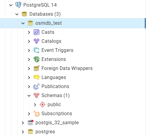
Figure 6 An illustration of the database named ‘osmdb_test’.

Note

• The parameter password is by default None. If we don’t specify a password for creating an instance, we’ll need to manually type in the password to the PostgreSQL server.

• The class PostgresOSM incorporates the classes for downloading and reading OSM data from the modules downloader and reader as properties. In the case of the above instance, osmdb.downloader is equivalent to the class GeofabrikDownloader, as the parameter data_source='Geofabrik' by default.

• To relate the instance osmdb_test to BBBike data, we could just run osmdb.data_source = 'BBBike'.

• See also the example of reading Birmingham shapefile data.

Import data into the database

To import any of the above OSM data to a database in the connected PostgreSQL server, we can use the method import_osm_data().

For example, let’s now try to import rutland_pbf_parsed_1 (see also the parsed PBF data of Rutland above that we’ve got from previous PBF data (.pbf / .osm.pbf) section:

>>> subregion_name = 'Rutland'

>>> osmdb.import_osm_data(
...     osm_data=rutland_pbf_parsed_1, table_name=subregion_name, schema_names=None,
...     verbose=True)
Proceed to import data into the table "Rutland" at postgres:***@localhost:5432/osmdb_test
? [No]|Yes: yes
Importing the data ...
  "points" ... Done: <total of rows> features.
  "lines" ... Done: <total of rows> features.
  "multilinestrings" ... Done: <total of rows> features.
  "multipolygons" ... Done: <total of rows> features.
  "other_relations" ... Done: <total of rows> features.

Note

• The parameter schema_names is by default None, meaning that we import all the available layers of the PBF data into the database.

In the example above, the schemas are ‘points’, ‘lines’, ‘multilinestrings’, ‘multipolygons’ and ‘other_relations’. If they do not exist, they are created in the database ‘osmdb_test’ when running the method import_osm_data(). Each of the schemas corresponds to a key (i.e. name of a layer) of rutland_pbf_parsed_1 (as illustrated in Figure 7); the data of each layer is imported into a table named as “Rutland” under the corresponding schema (as illustrated in Figure 8).

Figure 7 An illustration of schemas for importing OSM PBF data into a PostgreSQL database.

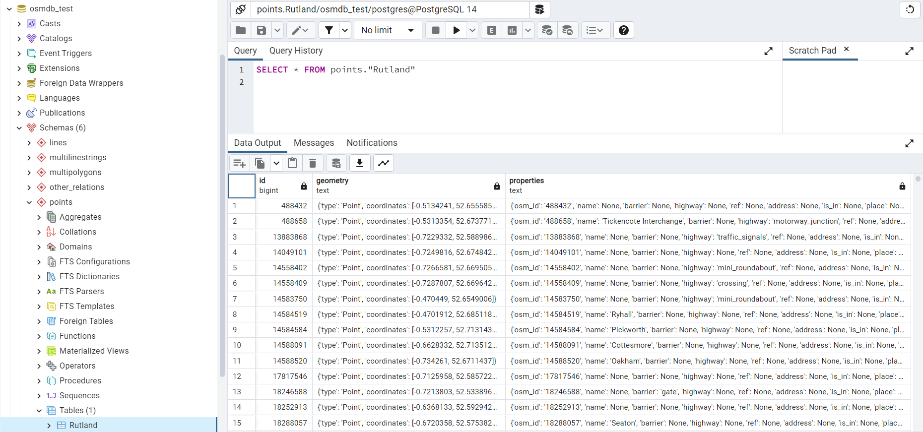
Figure 8 An illustration of table name for storing the ‘points’ layer of the OSM PBF data of Rutland.

Fetch data from the database

To retrieve all or specific layers of the imported data, we can use the fetch_data() method:

>>> # Retrieve all the PBF data being just imported
>>> rutland_pbf_parsed_1_ = osmdb.fetch_data(subregion_name, verbose=True)
Fetching the data of "Rutland" ...
  "points" ... Done.
  "lines" ... Done.
  "multilinestrings" ... Done.
  "multipolygons" ... Done.
  "other_relations" ... Done.

Check the data rutland_pbf_parsed_1_ we just retrieved:

>>> retr_data_type = type(rutland_pbf_parsed_1_)
>>> print(f'Data type of `rutland_pbf_parsed_1_`:\n  {retr_data_type}')
Data type of `rutland_pbf_parsed_1_`:
  <class 'dict'>

>>> retr_data_keys = list(rutland_pbf_parsed_1_.keys())
>>> print(f'The "keys" of `rutland_pbf_parsed_1_`:\n  {retr_data_keys}')
The "keys" of `rutland_pbf_parsed_1_`:
  ['points', 'lines', 'multilinestrings', 'multipolygons', 'other_relations']

>>> retr_layer_type = type(rutland_pbf_parsed_1_['points'])
>>> print(f'Data type of the corresponding layer:\n  {retr_layer_type}')
Data type of the corresponding layer:
  <class 'pandas.DataFrame'>

Take a quick look at the data of the ‘points’:

>>> rutland_pbf_parsed_1_points_ = rutland_pbf_parsed_1_['points']
>>> rutland_pbf_parsed_1_points_.head()
         id  ...                                         properties
0    488658  ...  {'osm_id': '488658', 'name': 'Tickencote Inter...
1  13883868  ...  {'osm_id': '13883868', 'name': None, 'barrier'...
2  14049101  ...  {'osm_id': '14049101', 'name': None, 'barrier'...
3  14558402  ...  {'osm_id': '14558402', 'name': None, 'barrier'...
4  14558409  ...  {'osm_id': '14558409', 'name': None, 'barrier'...
[5 rows x 3 columns]

Check whether rutland_pbf_parsed_1_ is equal to rutland_pbf_parsed_1 (see also the parsed data):

>>> # Check each of the layers:
>>> #   'points', 'lines', 'multilinestrings', 'multipolygons' or 'other_relations'
>>> check_equivalence = all(
...     rutland_pbf_parsed_1[lyr_name].equals(rutland_pbf_parsed_1_[lyr_name])
...     for lyr_name in rutland_pbf_parsed_1.keys())
>>> print(f"`rutland_pbf_parsed_1_` is equivalent to `rutland_pbf_parsed_1`: "
...       f"{check_equivalence}")
`rutland_pbf_parsed_1_` is equivalent to `rutland_pbf_parsed_1`: True

Note

• The parameter layer_names is None by default, meaning that we fetch data of all layers available from the database.

• The data stored in the database was parsed by the method GeofabrikReader.read_pbf() given expand=True (see the parsed data). When it is being imported in the PostgreSQL server, the data type of the column 'coordinates' is converted from list to str. Therefore, to retrieve the same data in the above example for the method fetch_data(), the parameter decode_geojson is by default True.

Specific layers of shapefile

Below is another example of importing/fetching data of multiple layers in a customised order. Let’s firstly import the transport-related layers of Leeds shapefile data.

Note

• 'Leeds' is not listed on the free download catalogue of Geofabrik but that of BBBike. We need to change the data source to 'BBBike' for the instance osmdb (see also the note above).

>>> osmdb.data_source = 'BBBike'  # Change to 'BBBike'

>>> subregion_name = 'Leeds'

>>> leeds_shp = osmdb.reader.read_shp(
...     subregion_name=subregion_name, data_dir=data_dir, download=True, verbose=True)
Downloading "Leeds.osm.shp.zip" 100%|██████████| 57.8M/57.8M | 18.0MB/s | ETA: 00:00
  Saving "Leeds.osm.shp.zip" to "./tests/osm_data/leeds/" ... Done.
Extracting "./tests/osm_data/leeds/Leeds.osm.shp.zip"
  to "./tests/osm_data/leeds/" ... Done.
Reading the shapefile(s) at "./tests/osm_data/leeds/Leeds-shp/shape/" ... Done.

Check the data leeds_shp:

>>> retr_data_type = type(leeds_shp)
>>> print(f'Data type of `leeds_shp`:\n  {retr_data_type}')
Data type of `leeds_shp`:
  <class 'dict'>

>>> retr_data_keys = list(leeds_shp.keys())
>>> print(f'The "keys" of `leeds_shp`:\n  {'\n  '.join(retr_data_keys)}')
The "keys" of `leeds_shp`:
  buildings
  landuse
  natural
  places
  points
  railways
  roads
  waterways

>>> leeds_shp_railways = leeds_shp['railways']
>>> retr_layer_type = type(leeds_shp_railways)
>>> print(f'Data type of the \'railways\' layer:\n  {retr_layer_type}')
Data type of the 'railways' layer:
  <class 'geopandas.geodataframe.GeoDataFrame'>

We could import the data of a list of selected layers. For example, let’s import the data of 'railways', 'roads' and 'waterways':

>>> layer_names = ['railways', 'roads', 'waterways']

>>> osmdb.import_osm_data(
...     leeds_shp, table_name=subregion_name, schema_names=layer_names, verbose=True)
Proceed to import data into the table "Leeds" at postgres:***@localhost:5432/osmdb_test
? [No]|Yes: yes
Importing the data ...
  "railways" ... Done: <total of rows> features.
  "roads" ... Done: <total of rows> features.
  "waterways" ... Done: <total of rows> features.

As illustrated in Figure 9, three schemas: ‘railways’, ‘roads’ and ‘waterways’ are created in the ‘osmdb_test’ database for storing the data of the three shapefile layers of Leeds.

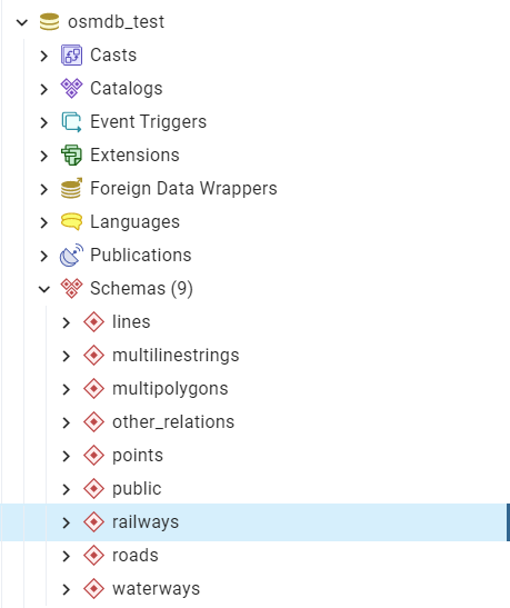
Figure 9 An illustration of the newly created schemas for the selected layers of Leeds shapefile data.

Now let’s fetch only the ‘railways’ data of Leeds from the ‘osmdb_test’ database:

>>> layer_name = 'railways'

>>> leeds_shp_ = osmdb.fetch_data(
...     subregion_name, layer_names=layer_name, sort_by='osm_id', verbose=True)
Fetching the data of "Leeds" ...
    "railways" ... Done.

Check the data leeds_shp_:

>>> retr_data_type = type(leeds_shp_)
>>> print(f'Data type of `leeds_shp_`:\n  {retr_data_type}')
Data type of `leeds_shp_`:
  <class 'dict'>

>>> retr_data_keys = list(leeds_shp_.keys())
>>> print(f'The "keys" of `leeds_shp_`:\n  {retr_data_keys}')
The "keys" of `leeds_shp_`:
  ['railways']

>>> # Data frame of the 'railways' layer
>>> leeds_shp_railways_ = leeds_shp_[layer_name]
>>> leeds_shp_railways_.head()
    osm_id  ...                                           geometry
0  3666100  ...  LINESTRING (-1.4935085 53.6772284, -1.4941684 ...
1  3688274  ...  LINESTRING (-1.5321838 53.6588828, -1.5316487 ...
2  3688277  ...  LINESTRING (-1.4361755 53.6908246, -1.4365117 ...
3  3688278  ...  LINESTRING (-1.4265919 53.6975115, -1.4268996 ...
4  3688279  ...  LINESTRING (-1.3564814 53.7237694, -1.3569774 ...
[5 rows x 4 columns]

Note

• The original leeds_shp_railways is a GeoDataFrame, however the retrieved leeds_shp_railways_ is a standard Pandas DataFrame.

• It must be noted that empty strings, '', may be automatically saved as None when importing leeds_shp into the PostgreSQL database.

• The data retrieved from a PostgreSQL database may not be in the same order as it is in the database; the retrieved leeds_shp_railways_ may not be exactly equal to leeds_shp_railways. However, they contain the same information. We can sort the data by 'osm_id' or 'id' and convert geometry to WKT/WKB (or vice versa) to make a comparison (see the test code below).

Check whether leeds_shp_railways_ is equivalent to leeds_shp_railways:

>>> import shapely.wkt
>>> import geopandas as gpd

>>> # Convert `leeds_shp_railways_` to a GeoDataFrame
>>> leeds_shp_railways_geo = leeds_shp_railways_.copy()
>>> leeds_shp_railways_geo['geometry'] = leeds_shp_railways_geo['geometry'].map(
...     shapely.wkt.loads)
>>> leeds_shp_railways_geo = gpd.GeoDataFrame(
...     leeds_shp_railways_geo, crs=osmdb.reader.SHP.EPSG4326_WGS84_PROJ4)

>>> check_eq = leeds_shp_railways_geo.equals(leeds_shp_railways)
>>> print(f"`leeds_shp_railways_geo` is equivalent to `leeds_shp_railways`: {check_eq}")
`leeds_shp_railways_geo` is equivalent to `leeds_shp_railways`: True

Drop data

To drop the data of all or selected layers that have been imported for one or multiple geographic regions, we can use the method drop_subregion_tables().

For example, let’s now drop the ‘railways’ schema for Leeds:

>>> # Recall that: subrgn_name == 'Leeds'; lyr_name == 'railways'
>>> osmdb.drop_subregion_tables(subregion_name, schema_names=layer_name, verbose=True)
Proceed to drop table "railways"."Leeds"
  from postgres:***@localhost:5432/osmdb_test
? [No]|Yes: yes
Dropping the table ...
  "railways"."Leeds" ... Done.

Then drop the ‘waterways’ schema for Leeds, and both the ‘lines’ and ‘multilinestrings’ schemas for Rutland:

>>> subregion_names = ['Leeds', 'Rutland']
>>> layer_names = ['waterways', 'lines', 'multilinestrings']
>>> osmdb.drop_subregion_tables(subregion_names, schema_names=layer_names, verbose=True)
Proceed to drop tables from postgres:***@localhost:5432/osmdb_test:
    "Leeds"
    "Rutland"
  under the schemas:
    "multilinestrings"
    "waterways"
    "lines"
? [No]|Yes: yes
Dropping the tables ...
  "multilinestrings"."Rutland" ... Done.
  "waterways"."Leeds" ... Done.
  "lines"."Rutland" ... Done.

We could also easily drop the whole database ‘osmdb_test’ if we don’t need it anymore:

>>> osmdb.drop_database(verbose=True)
Drop the database "osmdb_test" from postgres:***@localhost:5432?
 [No]|Yes: yes
Dropping "osmdb_test" ... Done.

Clear up ‘the mess’ in here

Now we are approaching the end of this tutorial. The final task we may want to do is to remove all the data files that have been downloaded and generated. Those data are all stored in the directory “tests/osm_data/”. Let’s take a quick look at what’s in here:

>>> os.listdir(data_dir)  # Recall that dat_dir == "tests/osm_data"
['birmingham',
 'greater-london',
 'leeds',
 'lon-bir-railways',
 'london',
 'rutland',
 'west-midlands',
 'west-yorkshire']

Let’s delete the directory “tests/osm_data/”:

>>> from pyhelpers.dirs import delete_dir

>>> delete_dir(data_dir, verbose=True)
To delete the directory "./tests/osm_data/" (Not empty)
? [No]|Yes: yes
Deleting "./tests/osm_data/" ... Done.

>>> os.path.isdir(data_dir)  # Check if the directory still exists
False

This is the end of the quick-start tutorial.

---

Any issues regarding the use of the package are all welcome and should be logged/reported onto the Issue Tracker.

For more details and examples, check subpackages and modules.