Tutorial
For a demonstration of how pydriosm works with OpenStreetMap (OSM) data, this part of the documentation provides a quick guide with some practical examples of using the package to implement tasks of downloading, parsing and storage I/O of the OSM data.
Note
All the data used in this quick-start tutorial will be downloaded and saved to a directory named “tests\osm_data\” (which will be created if it does not exist) at the current working directory.
At the end of the tutorial, you will be asked to confirm whether you would like to retain or remove the directory (i.e. “tests\osm_data\”). If yes, all the downloaded data and those generated during the tutorial will be deleted permanently.
Download data
The current release of the package works for the (sub)region-based OSM data extracts, which are available from the free download servers: Geofabrik and BBBike. To start with, let’s use the class GeofabrikDownloader from the module downloader to download a data file from the Geofabrik free download server.
>>> from pydriosm.downloader import GeofabrikDownloader
>>> # from pydriosm import GeofabrikDownloader

>>> # Create an instance for downloading the Geofabrik free data extracts
>>> gfd = GeofabrikDownloader()

>>> gfd.LONG_NAME  # Name of the data
'Geofabrik OpenStreetMap data extracts'

>>> gfd.FILE_FORMATS  # Available file formats
{'.osm.bz2', '.osm.pbf', '.shp.zip'}
To explore what data is available for download, you may check a download catalogue by using the method GeofabrikDownloader.get_catalogue():
>>> # A download catalogue for all subregions
>>> geofabrik_download_catalogue = gfd.get_catalogue()
>>> geofabrik_download_catalogue.head()
               subregion  ...                                           .osm.bz2
0                 Africa  ...  https://download.geofabrik.de/africa-latest.os...
1             Antarctica  ...  https://download.geofabrik.de/antarctica-lates...
2                   Asia  ...  https://download.geofabrik.de/asia-latest.osm.bz2
3  Australia and Oceania  ...  https://download.geofabrik.de/australia-oceani...
4        Central America  ...  https://download.geofabrik.de/central-america-...

[5 rows x 6 columns]
If we would like to download a protocolbuffer binary format (PBF) data file of a specific geographic region, we need to specify the name of the (sub)region and the file format (i.e. ".pbf" or ".osm.pbf"). For example, let’s try to download the PBF data of 'London' and save it to a directory "tests\\osm_data":
>>> subrgn_name = 'London'  # Name of a (sub)region; case-insensitive
>>> file_format = ".pbf"  # OSM data file format
>>> dwnld_dir = "tests\\osm_data"  # Name of or path to a directory where the data is saved

>>> # Download the OSM PBF data of London from Geofabrik download server
>>> gfd.download_osm_data(
...     subregion_names=subrgn_name, osm_file_format=file_format, download_dir=dwnld_dir,
...     verbose=True)
To download .osm.pbf data of the following geographic (sub)region(s):
    Greater London
? [No]|Yes: yes
Downloading "greater-london-latest.osm.pbf"
    to "tests\osm_data\greater-london\" ... Done.
Since the data has been successfully downloaded, it will not be downloaded again if you run the method given the same arguments:
>>> gfd.download_osm_data(
...     subregion_names=subrgn_name, osm_file_format=file_format, download_dir=dwnld_dir,
...     verbose=True)
"greater-london-latest.osm.pbf" is already available
    at "tests\osm_data\greater-london\".
Note
If the data file does not exist at the specified directory, we would need to confirm whether to proceed to download it as, by default,
confirmation_required=True. To skip the confirmation requirement, we could setconfirmation_required=False.The parameter
download_diris by defaultNone, in which case the downloaded data file is saved to the default data directory. For example, the default directory for in the case above should be “geofabrik\europe\great-britain\england\greater-london\”.After the downloading process completes, we can find the downloaded data file at “tests\osm_data\” and the (default) filename is greater-london-latest.osm.pbf.
The parameter
updateis by defaultFalse. When the data file already exists at the specified or default download directory and we setupdate=True, the method would replace the existing file with a freshly downloaded one.
If we would also like to have the path to the downloaded file, we could set ret_download_path=True. See the example below:
>>> path_to_london_pbf = gfd.download_osm_data(
...     subregion_names=subrgn_name, osm_file_format=file_format, download_dir=dwnld_dir,
...     update=True, verbose=2, ret_download_path=True)
"greater-london-latest.osm.pbf" is already available
    at "tests\osm_data\greater-london\".
To update the .osm.pbf data of the following geographic (sub)region(s):
    Greater London
? [No]|Yes: yes
Updating "greater-london-latest.osm.pbf"
    at "tests\osm_data\greater-london\" ...
"tests\osm_data\greater-london\greater-london-latest.osm.pbf": 82.9MB [00:01, 52.8MB/s]
Done.
In the example above, update=True allowed us to download the PBF data file again and replace the existing one. In addition, we also set verbose=2, which requires tqdm, to print more details about the downloading process.
Now let’s check the file path and the filename of the downloaded data:
>>> import os

>>> path_to_london_pbf_ = path_to_london_pbf[0]

>>> # Relative file path:
>>> print(f'Current (relative) file path: "{os.path.relpath(path_to_london_pbf_)}"')
Current (relative) file path: "tests\osm_data\greater-london\greater-london-latest.osm.pbf"

>>> # Default filename:
>>> london_pbf_filename = os.path.basename(path_to_london_pbf_)
>>> print(f'Default filename: "{london_pbf_filename}"')
Default filename: "greater-london-latest.osm.pbf"
Alternatively, you could also make use of the method .get_default_pathname() to get the default path to the data file (even when it does not exist):
We could also make use of the method get_default_pathname() to directly get the information (even if the file does not exist):
>>> download_info = gfd.get_valid_download_info(subrgn_name, file_format, dwnld_dir)
>>> subrgn_name_, london_pbf_filename, london_pbf_url, london_pbf_pathname = download_info
>>> print(f'Current (relative) file path: "{os.path.relpath(london_pbf_pathname)}"')
Current (relative) file path: "tests\osm_data\greater-london\greater-london-latest.osm.pbf"

>>> print(f'Default filename: "{london_pbf_filename}"')
Default filename: "greater-london-latest.osm.pbf"
In addition, we can also download the data of multiple (sub)regions at one go. For example, let’s now download the PBF data of both 'West Yorkshire' and 'West Midlands', and return their file paths:
>>> subrgn_names = ['West Yorkshire', 'West Midlands']
>>> paths_to_pbf = gfd.download_osm_data(
...     subregion_names=subrgn_names, osm_file_format=file_format, download_dir=dwnld_dir,
...     verbose=True, ret_download_path=True)
To download .osm.pbf data of the following geographic (sub)region(s):
    West Yorkshire
    West Midlands
? [No]|Yes: yes
Downloading "west-yorkshire-latest.osm.pbf"
    to "tests\osm_data\west-yorkshire\" ... Done.
Downloading "west-midlands-latest.osm.pbf"
    to "tests\osm_data\west-midlands\" ... Done.
Check the pathnames of the data files:
>>> for path_to_pbf in paths_to_pbf:
...     print(f"\"{os.path.relpath(path_to_pbf)}\"")
"tests\osm_data\west-yorkshire\west-yorkshire-latest.osm.pbf"
"tests\osm_data\west-midlands\west-midlands-latest.osm.pbf"
Read/parse data
To read/parse any of the downloaded data files above, we can use the class PBFReadParse or GeofabrikReader, which requires the python package GDAL.
PBF data (.pbf / .osm.pbf)
Now, let’s try to use the method GeofabrikReader.read_osm_pbf() to read the PBF data of the subregion 'Rutland':
>>> from pydriosm.reader import GeofabrikReader  # from pydriosm import GeofabrikReader

>>> # Create an instance for reading the downloaded Geofabrik data extracts
>>> gfr = GeofabrikReader()

>>> subrgn_name = 'Rutland'
>>> dat_dir = dwnld_dir  # i.e. "tests\\osm_data"

>>> rutland_pbf_raw = gfr.read_osm_pbf(
...     subregion_name=subrgn_name, data_dir=dat_dir, verbose=True)
Downloading "rutland-latest.osm.pbf"
    to "tests\osm_data\rutland\" ... Done.
Reading "tests\osm_data\rutland\rutland-latest.osm.pbf" ... Done.
Check the data types:
>>> raw_data_type = type(rutland_pbf_raw)
>>> print(f'Data type of `rutland_pbf_parsed`:\n\t{raw_data_type}')
Data type of `rutland_pbf_parsed`:
    <class 'dict'>

>>> raw_data_keys = list(rutland_pbf_raw.keys())
>>> print(f'The "keys" of `rutland_pbf_parsed`:\n\t{raw_data_keys}')
The "keys" of `rutland_pbf_parsed`:
    ['points', 'lines', 'multilinestrings', 'multipolygons', 'other_relations']

>>> raw_layer_data_type = type(rutland_pbf_raw['points'])
>>> print(f'Data type of the corresponding layer:\n\t{raw_layer_data_type}')
Data type of the corresponding layer:
    <class 'list'>

>>> raw_value_type = type(rutland_pbf_raw['points'][0])
>>> print(f'Data type of the individual feature:\n\t{raw_value_type}')
Data type of the individual feature:
    <class 'osgeo.ogr.Feature'>
As we see from the above, the variable rutland_pbf_raw is in dict type. It has five keys: 'points', 'lines', 'multilinestrings', 'multipolygons' and 'other_relations', each of which corresponds to the name of a layer of the PBF data.
However, the raw data is not human-readable. We can set readable=True to parse the individual features using GDAL.
Note
The method
GeofabrikReader.read_osm_pbf(), which relies on GDAL, may take tens of minutes (or even much longer) to parse a PBF data file, depending on the size of the data file.If the size of a data file is greater than the specified
chunk_size_limit(which defaults to50MB), the data will be parsed in a chunk-wise manner.
>>> # Set `readable=True`
>>> rutland_pbf_parsed_0 = gfr.read_osm_pbf(
...     subregion_name=subrgn_name, data_dir=dat_dir, readable=True, verbose=True)
Parsing "tests\osm_data\rutland\rutland-latest.osm.pbf" ... Done.
Check the data types:
>>> parsed_data_type = type(rutland_pbf_parsed_0)
>>> print(f'Data type of `rutland_pbf_parsed`:\n\t{parsed_data_type}')
Data type of `rutland_pbf_parsed`:
    <class 'dict'>

>>> parsed_data_keys = list(rutland_pbf_parsed_0.keys())
>>> print(f'The "keys" of `rutland_pbf_parsed`:\n\t{parsed_data_keys}')
The "keys" of `rutland_pbf_parsed`:
    ['points', 'lines', 'multilinestrings', 'multipolygons', 'other_relations']

>>> parsed_layer_type = type(rutland_pbf_parsed_0['points'])
>>> print(f'Data type of the corresponding layer:\n\t{parsed_layer_type}')
Data type of the corresponding layer:
    <class 'pandas.core.series.Series'>
Let’s further check out the 'points' layer as an example:
>>> rutland_pbf_points_0 = rutland_pbf_parsed_0['points']  # The layer of 'points'
>>> rutland_pbf_points_0.head()
0    {'type': 'Feature', 'geometry': {'type': 'Poin...
1    {'type': 'Feature', 'geometry': {'type': 'Poin...
2    {'type': 'Feature', 'geometry': {'type': 'Poin...
3    {'type': 'Feature', 'geometry': {'type': 'Poin...
4    {'type': 'Feature', 'geometry': {'type': 'Poin...
Name: points, dtype: object

>>> rutland_pbf_points_0_0 = rutland_pbf_points_0[0]  # A feature of the 'points' layer
>>> rutland_pbf_points_0_0
{'type': 'Feature',
 'geometry': {'type': 'Point', 'coordinates': [-0.5134241, 52.6555853]},
 'properties': {'osm_id': '488432',
  'name': None,
  'barrier': None,
  'highway': None,
  'ref': None,
  'address': None,
  'is_in': None,
  'place': None,
  'man_made': None,
  'other_tags': '"odbl"=>"clean"'},
 'id': 488432}
Each row (i.e. feature) of rutland_pbf_points_0 is GeoJSON data, which is a nested dictionary.
The charts (Fig. 1 - Fig. 5) below illustrate the different geometry types and structures (i.e. all keys within the corresponding GeoJSON data) for each layer:

Fig. 1 Type of the geometry object and keys within the nested dictionary of 'points'.

Fig. 2 Type of the geometry object and keys within the nested dictionary of 'lines'.

Fig. 3 Type of the geometry object and keys within the nested dictionary of 'multilinestrings'.

Fig. 4 Type of the geometry object and keys within the nested dictionary of 'multipolygons'.

Fig. 5 Type of the geometry object and keys within the nested dictionary of 'other_relations'.
If we set expand=True, we can transform the GeoJSON records to dataframe and obtain data of ‘visually’ (though not virtually) higher level of granularity (see also how to import the data into a PostgreSQL database):
>>> rutland_pbf_parsed_1 = gfr.read_osm_pbf(
...     subregion_name=subrgn_name, data_dir=dat_dir, expand=True, verbose=True)
Parsing "tests\osm_data\rutland\rutland-latest.osm.pbf" ... Done.
Data of the expanded 'points' layer (see also the retrieved data from database):
>>> rutland_pbf_points_1 = rutland_pbf_parsed_1['points']
>>> rutland_pbf_points_1.head()
         id  ...                                         properties
0    488432  ...  {'osm_id': '488432', 'name': None, 'barrier': ...
1    488658  ...  {'osm_id': '488658', 'name': 'Tickencote Inter...
2  13883868  ...  {'osm_id': '13883868', 'name': None, 'barrier'...
3  14049101  ...  {'osm_id': '14049101', 'name': None, 'barrier'...
4  14558402  ...  {'osm_id': '14558402', 'name': None, 'barrier'...

[5 rows x 3 columns]

>>> rutland_pbf_points_1['geometry'].head()
0    {'type': 'Point', 'coordinates': [-0.5134241, ...
1    {'type': 'Point', 'coordinates': [-0.5313354, ...
2    {'type': 'Point', 'coordinates': [-0.7229332, ...
3    {'type': 'Point', 'coordinates': [-0.7249816, ...
4    {'type': 'Point', 'coordinates': [-0.7266581, ...
Name: geometry, dtype: object
The data can be further transformed/parsed via three more parameters: parse_geometry, parse_other_tags and parse_properties, which all default to False.
For example, let’s now try expand=True and parse_geometry=True:
>>> rutland_pbf_parsed_2 = gfr.read_osm_pbf(
...     subrgn_name, data_dir=dat_dir, expand=True, parse_geometry=True, verbose=True)
>>> rutland_pbf_points_2 = rutland_pbf_parsed_2['points']
Parsing "tests\osm_data\rutland\rutland-latest.osm.pbf" ... Done.

>>> rutland_pbf_points_2['geometry'].head()
         id  ...                                         properties
0    488432  ...  {'osm_id': '488432', 'name': None, 'barrier': ...
1    488658  ...  {'osm_id': '488658', 'name': 'Tickencote Inter...
2  13883868  ...  {'osm_id': '13883868', 'name': None, 'barrier'...
3  14049101  ...  {'osm_id': '14049101', 'name': None, 'barrier'...
4  14558402  ...  {'osm_id': '14558402', 'name': None, 'barrier'...

[5 rows x 3 columns]

>>> rutland_pbf_points_2['geometry'].head()
0    POINT (-0.5134241 52.6555853)
1    POINT (-0.5313354 52.6737716)
2    POINT (-0.7229332 52.5889864)
3    POINT (-0.7249816 52.6748426)
4    POINT (-0.7266581 52.6695058)
Name: geometry, dtype: object
We can see the difference in 'geometry' column between rutland_pbf_points_1 and rutland_pbf_points_2.
Note
If only the name of a geographic (sub)region is provided, e.g.
rutland_pbf = gfr.read_osm_pbf(subregion_name='Rutland'), the method will go to look for the data file at the default file path. Otherwise, you need to specifydata_dirwhere the data file is.If the data file does not exist at the default or specified directory, the method will by default try to download it first. To give up downloading the data, setting
download=False.When
pickle_it=True, the parsed data will be saved as a Pickle file. When you run the method next time, it will try to load the Pickle file first, provided thatupdate=False(default); ifupdate=True, the method will try to download and parse the latest version of the data file. Note thatpickle_it=Trueworks only whenreadable=Trueand/orexpand=True.
Shapefiles (.shp.zip / .shp)
To read shapefile data, we can use the method GeofabrikReader.read_shp_zip() or SHPReadParse.read_shp(), which relies on PyShp (or optionally, GeoPandas.
Note
GeoPandas is not required for the installation of pydriosm.
For example, let’s now try to read the 'railways' layer of the shapefile of 'London' by using GeofabrikReader.read_shp_zip():
>>> subrgn_name = 'London'
>>> lyr_name = 'railways'

>>> london_shp = gfr.read_shp_zip(
...     subregion_name=subrgn_name, layer_names=lyr_name, data_dir=dat_dir, verbose=True)
Downloading "greater-london-latest-free.shp.zip"
    to "tests\osm_data\greater-london\" ... Done.
Extracting the following layer(s):
    'railways'
    from "tests\osm_data\greater-london\greater-london-latest-free.shp.zip"
      to "tests\osm_data\greater-london\greater-london-latest-free-shp\" ... Done.
Reading "tests\osm_data\greater-london\greater-london-latest-free-shp\gis_osm_railways_free_1...
Check the data:
>>> data_type = type(london_shp)
>>> print(f'Data type of `london_shp`:\n\t{data_type}')
Data type of `london_shp`:
    <class 'collections.OrderedDict'>

>>> data_keys = list(london_shp.keys())
>>> print(f'The "keys" of `london_shp`:\n\t{data_keys}')
The "keys" of `london_shp`:
    ['railways']

>>> layer_type = type(london_shp[lyr_name])
>>> print(f"Data type of the '{lyr_name}' layer:\n\t{layer_type}")
Data type of the 'railways' layer:
    <class 'pandas.core.frame.DataFrame'>
Similar to the parsed PBF data, london_shp is also in dict type, with the layer_name being its key by default.
>>> london_railways_shp = london_shp[lyr_name]  # london_shp['railways']
>>> london_railways_shp.head()
   osm_id  code  ...                                        coordinates shape_type
0   30804  6101  ...  [(0.0048644, 51.6279262), (0.0061979, 51.62926...          3
1  101298  6103  ...  [(-0.2249906, 51.493682), (-0.2251678, 51.4945...          3
2  101486  6103  ...  [(-0.2055497, 51.5195429), (-0.2051377, 51.519...          3
3  101511  6101  ...  [(-0.2119027, 51.5241906), (-0.2108059, 51.523...          3
4  282898  6103  ...  [(-0.1862586, 51.6159083), (-0.1868721, 51.613...          3

[5 rows x 9 columns]
Note
When
layer_name=None(default), all layers will be included.The parameter
feature_namesis related to'fclass'inlondon_railways_shp. You can specify one feature name (or multiple feature names) to get a subset oflondon_railways_shp.If the method
GeofabrikReader.read_shp_zip()could not find the target .shp file at the default or specified directory (i.e.dat_dir), it will try to extract the .shp file from the .shp.zip file.If the .shp.zip file is not available either, the method
GeofabrikReader.read_shp_zip()will try download the data first, provided thatdownload=True; otherwise, settingupdate=Truewould allow the method to download the latest version of the data despite the availability of the .shp.zip file.If you’d like to delete the .shp files and/or the downloaded .shp.zip file, set the parameters
rm_extracts=Trueand/orrm_shp_zip=True.
If we would like to combine multiple (sub)regions over a certain layer, we can use the method GeofabrikReader.merge_subregion_layer_shp() to concatenate the .shp files of the specific layer.
For example, let’s now merge the 'railways' layers of 'London' and 'Kent':
>>> subrgn_names = ['London', 'Kent']
>>> lyr_name = 'railways'

>>> path_to_merged_shp = gfr.merge_subregion_layer_shp(
...     subregion_names=subrgn_names, layer_name=lyr_name, data_dir=dat_dir, verbose=True,
...     ret_merged_shp_path=True)
"greater-london-latest-free.shp.zip" is already available
    at "tests\osm_data\greater-london\".
To download .shp.zip data of the following geographic (sub)region(s):
    Kent
? [No]|Yes: yes
Downloading "kent-latest-free.shp.zip"
    to "tests\osm_data\kent\" ... Done.
Merging the following shapefiles:
    "greater-london_gis_osm_railways_free_1.shp"
    "kent_gis_osm_railways_free_1.shp"
        In progress ... Done.
        Find the merged shapefile at "tests\osm_data\gre_lon-ken-railways\".

>>> # Relative path of the merged shapefile
>>> print(f"\"{os.path.relpath(path_to_merged_shp)}\"")
"tests\osm_data\gre_lon-ken-railways\linestring.shp"
We can read the merged shapefile data by using the method SHPReadParse.read_layer_shps():
>>> from pydriosm.reader import SHPReadParse  # from pydriosm import SHPReadParse

>>> london_kent_railways = SHPReadParse.read_layer_shps(path_to_merged_shp)
>>> london_kent_railways.head()
   osm_id  code  ...                                        coordinates shape_type
0   30804  6101  ...  [(0.0048644, 51.6279262), (0.0061979, 51.62926...          3
1  101298  6103  ...  [(-0.2249906, 51.493682), (-0.2251678, 51.4945...          3
2  101486  6103  ...  [(-0.2055497, 51.5195429), (-0.2051377, 51.519...          3
3  101511  6101  ...  [(-0.2119027, 51.5241906), (-0.2108059, 51.523...          3
4  282898  6103  ...  [(-0.1862586, 51.6159083), (-0.1868721, 51.613...          3

[5 rows x 9 columns]
For more details, also check out the methods SHPReadParse.merge_shps() and SHPReadParse.merge_layer_shps().
Import data into / fetch data from a PostgreSQL server
After downloading and reading the OSM data, pydriosm further provides a practical solution - the module pydriosm.ios - to managing the storage I/O of the data through database. Specifically, the class PostgresOSM, which inherits from pyhelpers.dbms.PostgreSQL, can assist us with importing the OSM data into, and retrieving it from, a PostgreSQL server.
To establish a connection with a PostgreSQL server, we need to specify the host address, port, username, password and a database name of the server. For example, let’s connect/create to a database named 'osmdb_test' in a local PostgreSQL server (as is installed with the default configuration):
>>> from pydriosm.ios import PostgresOSM

>>> host = 'localhost'
>>> port = 5432
>>> username = 'postgres'
>>> password = None  # You need to type it in manually if `password=None`
>>> database_name = 'osmdb_test'

>>> # Create an instance of a running PostgreSQL server
>>> osmdb = PostgresOSM(
...     host=host, port=port, username=username, password=password,
...     database_name=database_name, data_source='Geofabrik')
Password (postgres@localhost:5432): ***
Creating a database: "osmdb_test" ... Done.
Connecting postgres:***@localhost:5432/osmdb_test ... Successfully.
The example is illustrated in Fig. 6:
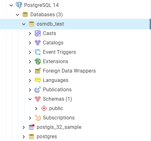
Fig. 6 An illustration of the database named ‘osmdb_test’.
Note
The parameter
passwordis by defaultNone. If we don’t specify a password for creating an instance, we’ll need to manually type in the password to the PostgreSQL server.The class
PostgresOSMincorporates the classes for downloading and reading OSM data from the modulesdownloaderandreaderas properties. In the case of the above instance,osmdb.downloaderis equivalent to the classGeofabrikDownloader, as the parameterdata_source='Geofabrik'by default.To relate the instance
osmdb_testto BBBike data, we could just runosmdb.data_source = 'BBBike'.See also the example of reading Birmingham shapefile data.
Import data into the database
To import any of the above OSM data to a database in the connected PostgreSQL server, we can use the method import_osm_data() or import_subregion_osm_pbf().
For example, let’s now try to import rutland_pbf_parsed_1 (see also the parsed PBF data of Rutland above that we’ve got from previous PBF data (.pbf / .osm.pbf) section:
>>> subrgn_name = 'Rutland'

>>> osmdb.import_osm_data(
...     rutland_pbf_parsed_1, table_name=subrgn_name, schema_names=None, verbose=True)
To import data into table "Rutland" at postgres:***@localhost:5432/osmdb_test
? [No]|Yes: yes
Importing the data ...
    "points" ... Done: <total of rows> features.
    "lines" ... Done: <total of rows> features.
    "multilinestrings" ... Done: <total of rows> features.
    "multipolygons" ... Done: <total of rows> features.
    "other_relations" ... Done: <total of rows> features.
Note
The parameter
schema_namesis by defaultNone, meaning that we import all the five layers of the PBF data into the database.
In the example above, five schemas are ‘points’, ‘lines’, ‘multilinestrings’, ‘multipolygons’ and ‘other_relations’. If they do not exist, they will be created in the database ‘osmdb_test’ when running the method import_osm_data(). Each of the schemas corresponds to a key (i.e. name of a layer) of rutland_pbf_parsed_1 (as illustrated in Fig. 7); the data of each layer is imported into a table named as “Rutland” under the corresponding schema (as illustrated in Fig. 8).
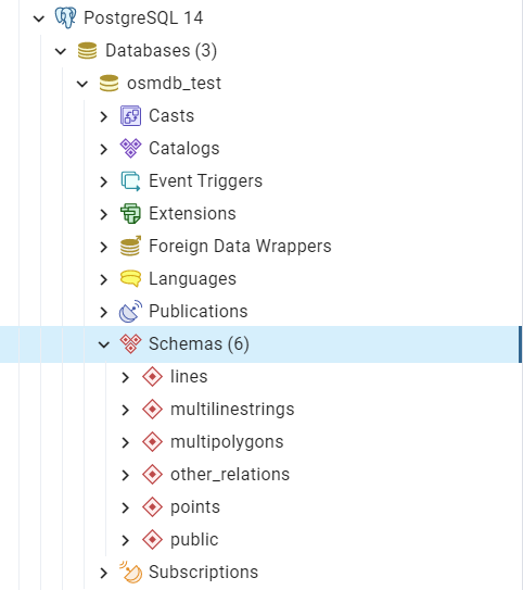
Fig. 7 An illustration of schemas for importing OSM PBF data into a PostgreSQL database.
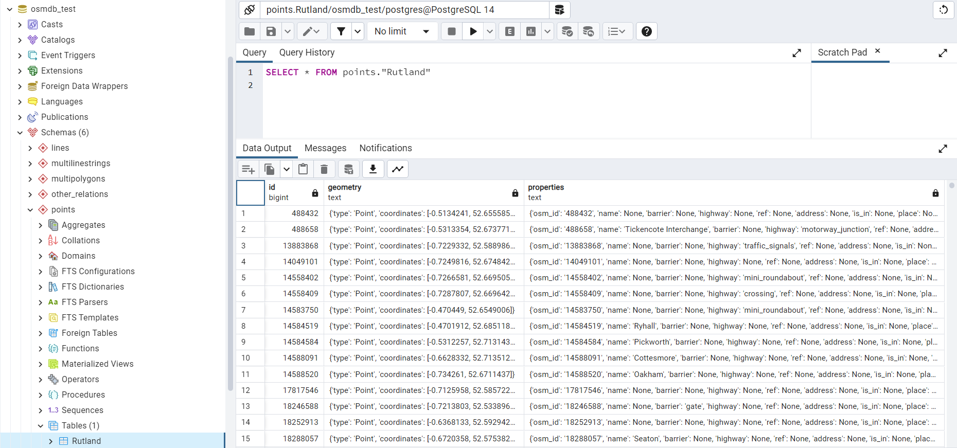
Fig. 8 An illustration of table name for storing the ‘points’ layer of the OSM PBF data of Rutland.
Fetch data from the database
To fetch all or specific layers of the imported data, we can use the method fetch_osm_data(). For example, let’s retrieve all the PBF data of Rutland with layer_names=None (by default):
>>> # Retrieve the data from the database
>>> rutland_pbf_parsed_1_ = osmdb.fetch_osm_data(subrgn_name, verbose=True)
Fetching the data of "Rutland" ...
    "points" ... Done.
    "lines" ... Done.
    "multilinestrings" ... Done.
    "multipolygons" ... Done.
    "other_relations" ... Done.
Check the data rutland_pbf_parsed_1_ we just retrieved:
>>> retr_data_type = type(rutland_pbf_parsed_1_)
>>> print(f'Data type of `rutland_pbf_parsed_1_`:\n\t{retr_data_type}')
Data type of `rutland_pbf_parsed_1_`:
    <class 'collections.OrderedDict'>

>>> retr_data_keys = list(rutland_pbf_parsed_1_.keys())
>>> print(f'The "keys" of `rutland_pbf_parsed_1_`:\n\t{retr_data_keys}')
The "keys" of `rutland_pbf_parsed_1_`:
    ['points', 'lines', 'multilinestrings', 'multipolygons', 'other_relations']

>>> retr_layer_type = type(rutland_pbf_parsed_1_['points'])
>>> print(f'Data type of the corresponding layer:\n\t{retr_layer_type}')
Data type of the corresponding layer:
    <class 'pandas.core.frame.DataFrame'>
Take a quick look at the data of the ‘points’:
>>> rutland_pbf_parsed_1_points_ = rutland_pbf_parsed_1_['points']
>>> rutland_pbf_parsed_1_points_.head()
         id  ...                                         properties
0    488432  ...  {'osm_id': '488432', 'name': None, 'barrier': ...
1    488658  ...  {'osm_id': '488658', 'name': 'Tickencote Inter...
2  13883868  ...  {'osm_id': '13883868', 'name': None, 'barrier'...
3  14049101  ...  {'osm_id': '14049101', 'name': None, 'barrier'...
4  14558402  ...  {'osm_id': '14558402', 'name': None, 'barrier'...

[5 rows x 3 columns]
Check whether rutland_pbf_parsed_1_ is equal to rutland_pbf_parsed_1 (see the parsed data):
>>> # 'points', 'lines', 'multilinestrings', 'multipolygons' or 'other_relations'
>>> lyr_name = 'points'

>>> check_equivalence = all(
...     rutland_pbf_parsed_1[lyr_name].equals(rutland_pbf_parsed_1_[lyr_name])
...     for lyr_name in rutland_pbf_parsed_1.keys())
>>> print(f"`rutland_pbf_parsed_` is equivalent to `rutland_pbf_parsed`: {check_equivalence}")
`rutland_pbf_parsed_` is equivalent to `rutland_pbf_parsed`: True
Note
The parameter
layer_namesisNoneby default, meaning that we fetch data of all layers available from the database.The data stored in the database was parsed by the method
GeofabrikReader.read_osm_pbf()givenexpand=True(see the parsed data). When it is being imported in the PostgreSQL server, the data type of the column'coordinates'is converted from list to str. Therefore, to retrieve the same data in the above example for the methodfetch_osm_data(), the parameterdecode_geojsonis by defaultTrue.
Specific layers of shapefile
Below is another example of importing/fetching data of multiple layers in a customised order. Let’s firstly import the transport-related layers of Birmingham shapefile data.
Note
>>> osmdb.data_source = 'BBBike'  # Change to 'BBBike'

>>> subrgn_name = 'Birmingham'

>>> bham_shp = osmdb.reader.read_shp_zip(subrgn_name, data_dir=dat_dir, verbose=True)
Downloading "Birmingham.osm.shp.zip"
    to "tests\osm_data\birmingham\" ... Done.
Extracting "tests\osm_data\birmingham\Birmingham.osm.shp.zip"
    to "tests\osm_data\birmingham\" ... Done.
Reading the shapefile(s) at
    "tests\osm_data\birmingham\Birmingham-shp\shape\" ... Done.
Check the data bham_shp:
>>> retr_data_type = type(bham_shp)
>>> print(f'Data type of `bham_shp`:\n\t{retr_data_type}')
Data type of `bham_shp`:
    <class 'collections.OrderedDict'>

>>> retr_data_keys = list(bham_shp.keys())
>>> print(f'The "keys" of `bham_shp`:\n\t{retr_data_keys}')
The "keys" of `bham_shp`:
    ['buildings', 'landuse', 'natural', 'places', 'points', 'railways', 'roads', 'waterways']

>>> retr_layer_type = type(bham_shp[lyr_name])
>>> print(f'Data type of the corresponding layer:\n\t{retr_layer_type}')
Data type of the corresponding layer:
    <class 'pandas.core.frame.DataFrame'>
We could import the data of a list of selected layers. For example, let’s import the data of 'railways', 'roads' and 'waterways':
>>> lyr_names = ['railways', 'roads', 'waterways']

>>> osmdb.import_osm_data(
...     bham_shp, table_name=subrgn_name, schema_names=lyr_names, verbose=True)
To import data into table "Birmingham" at postgres:***@localhost:5432/osmdb_test
? [No]|Yes: yes
Importing the data ...
    "railways" ... Done: <total of rows> features.
    "roads" ... Done: <total of rows> features.
    "waterways" ... Done: <total of rows> features.
As illustrated in Fig. 9, three schemas: ‘railways’, ‘roads’ and ‘waterways’ are created in the ‘osmdb_test’ database for storing the data of the three shapefile layers of Birmingham.
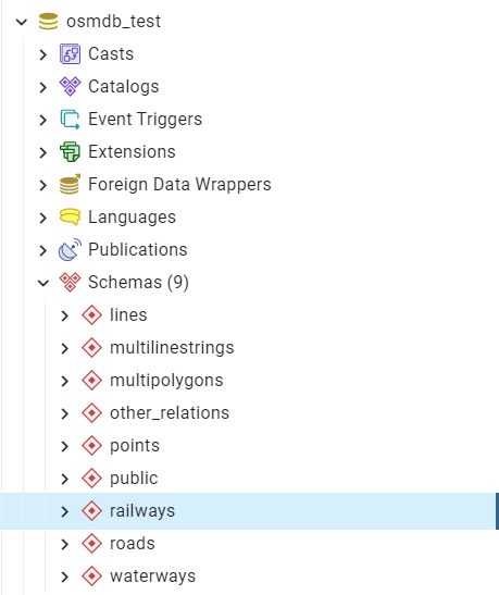
Fig. 9 An illustration of the newly created schemas for the selected layers of Birmingham shapefile data.
Now let’s fetch only the ‘railways’ data of Birmingham from the ‘osmdb_test’ database:
>>> lyr_name = 'railways'

>>> bham_shp_ = osmdb.fetch_osm_data(
...     subrgn_name, layer_names=lyr_name, sort_by='osm_id', verbose=True)
Fetching the data of "Birmingham" ...
    "railways" ... Done.
Check the data bham_shp_:
>>> retr_data_type = type(bham_shp_)
>>> print(f'Data type of `bham_shp_`:\n\t{retr_data_type}')
Data type of `bham_shp_`:
    <class 'collections.OrderedDict'>

>>> retr_data_keys = list(bham_shp_.keys())
>>> print(f'The "keys" of `bham_shp_`:\n\t{retr_data_keys}')
The "keys" of `bham_shp_`:
    ['railways']

>>> # Data frame of the 'railways' layer
>>> bham_shp_railways_ = bham_shp_[lyr_name]
>>> bham_shp_railways_.head()
    osm_id  ... shape_type
0      740  ...          3
1     2148  ...          3
2  2950000  ...          3
3  3491845  ...          3
4  3981454  ...          3

[5 rows x 5 columns]
Note
bham_shp_railwaysandbham_shp_railways_both in pandas.DataFrame type.It must be noted that empty strings,
'', may be automatically saved asNonewhen importingbham_shpinto the PostgreSQL database.The data retrieved from a PostgreSQL database may not be in the same order as it is in the database; the retrieved
bham_shp_railways_may not be exactly equal to bham_shp_railways. However, they contain exactly the same information. We could sort the data by'id'(or'osm_id') to make a comparison (see the test code below).
Check whether bham_shp_railways_ is equivalent to bham_shp_railways (before filling None with ''):
>>> bham_shp_railways = bham_shp[lyr_name]

>>> check_eq = bham_shp_railways_.equals(bham_shp_railways)
>>> print(f"`bham_shp_railways_` is equivalent to `bham_shp_railways`: {check_eq}")
`bham_shp_railways_` is equivalent to `bham_shp_railways`: False
Let’s fill None values with '' and check the equivalence again:
>>> # Try filling `None` values with `''`
>>> bham_shp_railways_.fillna('', inplace=True)

>>> # Check again whether `birmingham_shp_railways_` is equal to `birmingham_shp_railways`
>>> check_eq = bham_shp_railways_.equals(bham_shp_railways)
>>> print(f"`bham_shp_railways_` is equivalent to `bham_shp_railways`: {check_eq}")
`bham_shp_railways_` is equivalent to `bham_shp_railways`: True
Drop data
To drop the data of all or selected layers that have been imported for one or multiple geographic regions, we can use the method drop_subregion_tables().
For example, let’s now drop the ‘railways’ schema for Birmingham:
>>> # Recall that: subrgn_name == 'Birmingham'; lyr_name == 'railways'
>>> osmdb.drop_subregion_tables(subrgn_name, schema_names=lyr_name, verbose=True)
To drop table "railways"."Birmingham"
  from postgres:***@localhost:5432/osmdb_test
? [No]|Yes: yes
Dropping the table ...
    "railways"."Birmingham" ... Done.
Then drop the ‘waterways’ schema for Birmingham, and both the ‘lines’ and ‘multilinestrings’ schemas for Rutland:
>>> subrgn_names = ['Birmingham', 'Rutland']
>>> lyr_names = ['waterways', 'lines', 'multilinestrings']
>>> osmdb.drop_subregion_tables(subrgn_names, schema_names=lyr_names, verbose=True)
To drop tables from postgres:***@localhost:5432/osmdb_test:
    "Birmingham"
    "Rutland"
  under the schemas:
    "lines"
    "waterways"
    "multilinestrings"
? [No]|Yes: yes
Dropping the tables ...
    "lines"."Rutland" ... Done.
    "waterways"."Birmingham" ... Done.
    "multilinestrings"."Rutland" ... Done.
We could also easily drop the whole database ‘osmdb_test’ if we don’t need it anymore:
>>> osmdb.drop_database(verbose=True)
To drop the database "osmdb_test" from postgres:***@localhost:5432
? [No]|Yes: yes
Dropping "osmdb_test" ... Done.
Clear up ‘the mess’ in here
Now we are approaching the end of this tutorial. The final task we may want to do is to remove all the data files that have been downloaded and generated. Those data are all stored in the directory “tests\osm_data\”. Let’s take a quick look at what’s in here:
>>> os.listdir(dat_dir)  # Recall that dat_dir == "tests\\osm_data"
['birmingham',
 'greater-london',
 'gre_lon-ken-railways',
 'kent',
 'rutland',
 'west-midlands',
 'west-yorkshire']
Let’s delete the directory “tests\osm_data\”:
>>> from pyhelpers.dirs import delete_dir

>>> delete_dir(dat_dir, verbose=True)
To delete the directory "tests\osm_data\" (Not empty)
? [No]|Yes: yes
Deleting "tests\osm_data\" ... Done.

>>> os.path.exists(dat_dir)  # Check if the directory still exists
False
This is the end of the Tutorial.
Any issues regarding the use of the package are all welcome and should be logged/reported onto the Bug Tracker.
For more details and examples, check Modules.